Cell type deconvoluation & ST velocity

Key APIs

• expDeconv

• expVeloImp

External packages:

scvelo

Data download

Input data can be downloaded from Mouse_brain.tar.gz, please extract it with

tar -xzvf Mouse_brain.tar.gz

and change the variables RNA_PATH and ST_PATH in the next cell accordingly.

I. Cell type deconvoluation

Translate cell types from single cell reference to ST data (full-rank cluster mode)

• In addition to shared genes, TransDeconv requires single cell type lables and per-cell annotations as input;

• After fitting the translation function, TransDeconv will output the predictions as well as the weights for each cell type

preds, weight = expDeconv(
            adata_ref=rna_adata,
            adata_tgt=HybISS,
            seed=seed,
            device=device
            )

import scvelo as scv
import scanpy as sc
import numpy as np
import pandas as pd
from transpa.util import expVeloImp, leiden_cluster, expDeconv, build_adata, run_velocity
import torch
import warnings

print(scv.__version__)
print(sc.__version__)
warnings.filterwarnings('ignore')

seed = 10
device = torch.device("cuda:0") if torch.cuda.is_available() else torch.device("cpu")
# load preprocessed scRNA-seq and spatial datasets
RNA_PATH = 'Mouse_brain/RNA_adata.h5ad'
ST_PATH = 'Mouse_brain/HybISS_adata.h5ad'
RNA = sc.read_h5ad(RNA_PATH)
HybISS = sc.read_h5ad(ST_PATH)
RNA, HybISS

0.3.4
1.11.5

(AnnData object with n_obs × n_vars = 40733 × 16907
     obs: 'CellID', 'Age', 'Region', 'Tissue', 'Class', 'Subclass', 'initial_size_spliced', 'initial_size_unspliced', 'initial_size', 'n_counts'
     var: 'GeneName', 'gene_count_corr'
     layers: 'spliced', 'unspliced',
 AnnData object with n_obs × n_vars = 4628 × 119
     obs: 'n_counts'
     var: 'GeneName'
     obsm: 'X_xy_loc', 'xy_loc')

The following code prepares input for expDeconv, it

• filters SC types with less than 2 samples

• prepare cell cluster labels and annotations

sc.pp.pca(HybISS, n_comps=30)
celltype_counts = RNA.obs['Class'].value_counts()

celltype_drop = celltype_counts.index[celltype_counts < 2]
rna_adata = RNA.copy()
if len(celltype_drop):
    print(f'Drop celltype {list(celltype_drop)} (contain less 2 samples)')
    rna_adata = RNA[~RNA.obs['Class'].isin(celltype_drop),].copy()

classes = rna_adata.obs.Class.values
ct_list = np.unique(classes)

• Run the main cell type deconvoluation method

• Normalize result and select the top1 cell type

preds, weight = expDeconv(
            adata_ref=rna_adata,
            adata_tgt=HybISS,
            label_key='Class',
            seed=seed,
            device=device
            )

df_results = pd.DataFrame(weight, columns=ct_list)

df_results = (df_results.T/df_results.sum(axis=1)).T

HybISS.obs['Class'] = df_results.columns[np.argmax(df_results.values, axis=1)]

[expDeconv] 40733 ref cells, 4628 tgt spots, 19 cell types, 117 shared genes
[expDeconv] Auto-detected raw counts: False
[expDeconv] Selected 117 marker genes (topk=50, 19 cell types)
[expDeconv] Leiden clustering: 28 clusters
[expDeconv] Augmented target with cluster means -> 4656 total rows (4628 original spots)
[expDeconv] Score-init weights computed (4656 spots x 19 cell types)
[expDeconv] Starting fit_deconv (n_epochs=8000, lr=0.01, wd=0.001, wt_js=2.0)
  [fit_deconv] Epoch 1000/8000, loss: 6.937523
  [fit_deconv] Epoch 2000/8000, loss: 3.534264
  [fit_deconv] Epoch 3000/8000, loss: 2.646825
  [fit_deconv] Epoch 4000/8000, loss: 2.290432
  [fit_deconv] Epoch 5000/8000, loss: 2.118853
  [fit_deconv] Epoch 6000/8000, loss: 2.031667
  [fit_deconv] Epoch 7000/8000, loss: 1.992047
  [fit_deconv] Epoch 8000/8000, loss: 1.984471
[expDeconv] Training complete
[expDeconv] Prediction done: 4656 spots x 117 cell types

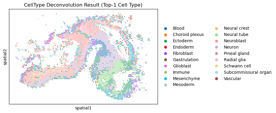
Plot the deconvolution result

HybISS.obsm['spatial'] = HybISS.obsm['X_xy_loc'] * np.array([[1, -1]])
sc.pl.spatial(HybISS, color='Class', title="CellType Deconvolution Result (Top-1 Cell Type)", spot_size=0.8)

II. RNA velocity imputation

Translate spliced and unspliced count matrices from SC to ST domain (Low-rank cell mode), before applying velocity estimation methods.

• Provide adata_raw (pre-normalisation AnnData) so that S/U are extracted automatically

• Output is imputed Spliced, Unspliced and other related matrices

res = expVeloImp(
            adata_ref=RNA,
            adata_tgt=HybISS,
            test_gene=RNA.var_names,
            signature_mode='cluster',
            n_epochs=2000,
            seed=seed,
            device=device,
            adata_raw=RNA_raw)
S, U, V, X = res

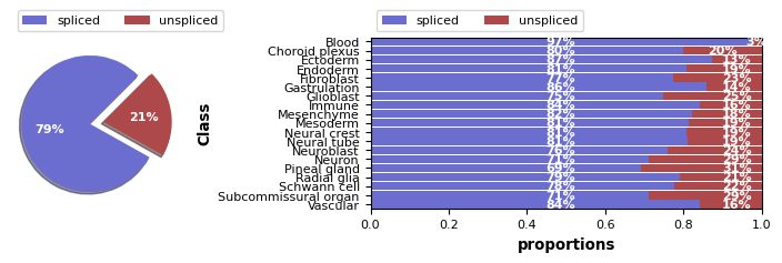
Check spliced and unspliced expressions

scv.pl.proportions(RNA, 'Class')

RNA_raw = RNA.copy()
scv.pp.filter_and_normalize(RNA, retain_genes=HybISS.var_names)

WARNING: Did not normalize X as it looks processed already. To enforce normalization, set `enforce=True`.
WARNING: Did not normalize spliced as it looks processed already. To enforce normalization, set `enforce=True`.
WARNING: Did not normalize unspliced as it looks processed already. To enforce normalization, set `enforce=True`.

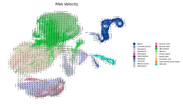
SC RNA Velocity

run_velocity(RNA, mode='stochastic')
scv.pl.velocity_embedding_grid(RNA,
                                vkey="stc_velocity",
                                basis='X_umap', color="Class",
                                legend_fontsize=5,
                                size=50,
                                legend_loc='right',
                                arrow_length=2,
                                dpi=100,
                                title='RNA Velocity')

computing neighbors
    finished (0:00:23) --> added
    'distances' and 'connectivities', weighted adjacency matrices (adata.obsp)
computing moments based on connectivities
    finished (0:01:17) --> added
    'Ms' and 'Mu', moments of un/spliced abundances (adata.layers)
computing velocities
    finished (0:04:04) --> added
    'stc_velocity', velocity vectors for each individual cell (adata.layers)
computing velocity graph (using 10/96 cores)
WARNING: Unable to create progress bar. Consider installing `tqdm` as `pip install tqdm` and `ipywidgets` as `pip install ipywidgets`,
or disable the progress bar using `show_progress_bar=False`.
    finished (0:02:59) --> added
    'stc_velocity_graph', sparse matrix with cosine correlations (adata.uns)
--> added 'stc_velocity_length' (adata.obs)
--> added 'stc_velocity_confidence' (adata.obs)
--> added 'stc_velocity_confidence_transition' (adata.obs)
computing velocity embedding
    finished (0:00:12) --> added
    'stc_velocity_umap', embedded velocity vectors (adata.obsm)

Prepare data

print(f'RNA: {RNA.shape}, HybISS: {HybISS.shape}')

RNA: (40733, 16907), HybISS: (4628, 119)

Run main imputation method for ST velocity estimation

res = expVeloImp(
            adata_ref=RNA,
            adata_tgt=HybISS,
            test_gene=RNA.var_names,
            signature_mode='cell',
            mapping_mode='lowrank',
            classes=classes,
            ct_list=ct_list,
            label_key='Class',
            n_epochs=1000,
            seed=seed,
            device=device,
            adata_raw=RNA_raw)
S, U, V, X = res

Organize new anndata for imputation result

imp_adata = build_adata(S, U, X, HybISS, RNA)
run_velocity(imp_adata)

computing neighbors
    finished (0:00:00) --> added
    'distances' and 'connectivities', weighted adjacency matrices (adata.obsp)
Normalized count data: X, spliced, unspliced.
computing moments based on connectivities
    finished (0:00:07) --> added
    'Ms' and 'Mu', moments of un/spliced abundances (adata.layers)
computing velocities
    finished (0:00:11) --> added
    'stc_velocity', velocity vectors for each individual cell (adata.layers)
computing velocity graph (using 10/96 cores)
    finished (0:00:24) --> added
    'stc_velocity_graph', sparse matrix with cosine correlations (adata.uns)
--> added 'stc_velocity_length' (adata.obs)
--> added 'stc_velocity_confidence' (adata.obs)
--> added 'stc_velocity_confidence_transition' (adata.obs)

AnnData object with n_obs × n_vars = 4627 × 16907
    obs: 'n_counts', 'Class', 'leiden', 'initial_size_unspliced', 'initial_size_spliced', 'initial_size', 'stc_velocity_self_transition', 'stc_velocity_length', 'stc_velocity_confidence', 'stc_velocity_confidence_transition'
    var: 'gene_count_corr', 'mean', 'std', 'stc_velocity_gamma', 'stc_velocity_qreg_ratio', 'stc_velocity_r2', 'stc_velocity_genes'
    uns: 'pca', 'Class_colors', 'neighbors', 'umap', 'leiden', 'stc_velocity_params', 'stc_velocity_graph', 'stc_velocity_graph_neg'
    obsm: 'X_xy_loc', 'xy_loc', 'X_pca', 'spatial', 'X_umap'
    layers: 'spliced', 'unspliced', 'Ms', 'Mu', 'stc_velocity', 'variance_stc_velocity'
    obsp: 'distances', 'connectivities'

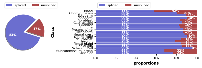
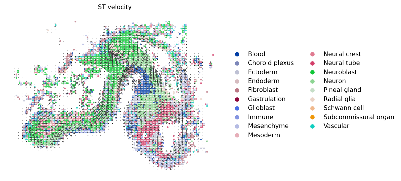
Ploting ST velocity

scv.pl.proportions(imp_adata, 'Class')

scv.pl.velocity_embedding_grid(imp_adata,
                                vkey="stc_velocity",
                                basis='xy_loc', color="Class",
                                legend_loc='right',
                                scale=0.5,
                                arrow_size=1.5,
                                arrow_length=2,
                                size=30,
                                alpha=0.8,
                                dpi=150,
                                title='ST velocity')

computing velocity embedding
    finished (0:00:01) --> added
    'stc_velocity_xy_loc', embedded velocity vectors (adata.obsm)